
OpenGL GLSL Texturing and Lighting
In this article I will demonstrate how to apply 2D textures to your 3D models. I will also show how to define lights that are used to illuminate the objects in your scene.
I assume that the reader has a basic knowledge of C++ and how to create and compile C++ programs. If you have never created an OpenGL program, then I suggest that you read my previous article titled [Introduction to OpenGL and GLSL] before continuing with this article.
Introduction
Texturing an object is the process of mapping a 2D (or sometimes 3D) image onto a 3D model so that you can achieve much higher detail in the model without using a lot of vertices. Without textures the only way to acquire the level of detail that can be achieved using texture mapping would be to specify a different colored vertex for each pixel of the screen. As you can imagine, adding detail to a model in this way can be very inefficient.
Lighting is required to set the mood for a scene. Lighting also provides a cue to the eye what the direction and shape of an object has. With the correct use of lighting we can make a scene dark and gloomy or bright and cheery.
Materials are used to determine how the light interacts with the surface of the model. A model can appear very shiny or very dull depending on the material properties of the model.
In this article, I will describe how to apply texturing, lighting and materials using OpenGL and GLSL.
Dependencies
For this article, I will rely on several 3rd party libraries to simplify programming.
- Free OpenGL Utility Toolkit (FreeGLUT 2.8.1): FreeGLUT is an open-source alternative to the OpenGL Utility Toolkit (GLUT) library. The purpose of the GLUT library is to provide window, keyboard, and mouse functionality in a platform-independent way.
- OpenGL Extension Wrangler (GLEW 1.10.0): The OpenGL Extension Wrangler library provides accessibility to the OpenGL core and extensions that may not be available in the OpenGL header files and libraries provided by your compiler.
- OpenGL Math Library (GLM 0.9.5): The OpenGL math library is written to be consistent with the math primitives provided by the GLSL shading language. This makes writing math functions in C++ very similar to the math functions you will see in GLSL shader code.
- SOIL: The Simple OpenGL Image Library is the easiest way that I am currently aware of to load textures into OpenGL. With a single method, you can load textures and get an OpenGL texture object. You can get the latest version of SOIL here: http://www.lonesock.net/soil.html
The Simple OpenGL Image Library provided from the link above had some issues when using it with an OpenGL 3.0 or higher forward-compatible context when it queries for extension support. I fixed this issue and provided a solution and project files for Visual Studio 2012 (vs11) that you can use for your own projects. You can download the updated version of SOIL here:
Texturing
Texture mapping is the process of applying a 2D (or 3D) image to a 3D model. Textures can provide much more detail to the model that would otherwise only be possible by creating models with a huge number of vertices. In order to correctly map the texture to a model we must specify a texture coordinate to each vertex of the model. A texture coordinate can be either be a single scalar in the case of 1D textures (a single row of texels which may represent a gradient, opacity or weight), a 2-component value in the case of 2D textures, or a 3-component value in the case of 3D textures or even a 4-component value in the case of projected textures. In this article I will only show applying 2D textures using 2-component texture coordinates.
Computing the correct texture coordinate for a vertex can be a complex process and it usually the job of the 3D modeling artists to generate the correct texture coordinates in a 3D content creation program like 3D Studio Max, Maya, or Blender.
The texture coordinate determines what texel is sampled from the texture. When dealing with 2D textures, the axis along the width of the texture is usually referred to as the U (or s coordinate) axis and the axis along the height of the texture is usually referred to as the V (or t coordinate) axis. For this reason, texture mapping can also be called “UV mapping”.
Texture coordinates are usually normalized in the range 0 to 1 in each axis. Normalized texture coordinates are useful because we may not always know the size of the texture in advance (and when using MIP maps, the size of the texture will actually change depending on the view of the object being textured).
The image below shows the texture coordinates and the corresponding axes that are used to refer to the texels.
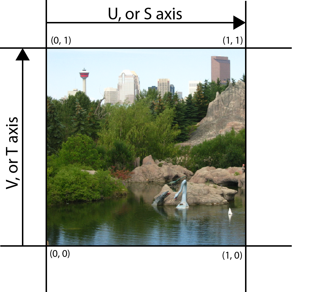
OpenGL Texture Coordinates
Loading Textures
Since there are so many different image formats, I will not go into much detail about how to load textures into memory. Instead, I will stick to the simple OpenGL image library (SOIL) for loading textures into graphics memory. SOIL is a free, open source image library that can load images from multiple image formats. If you are using OpenGL 3.0 or higher forward-compatible context, make sure you download the version of SOIL that I provide in the Dependency section above otherwise you will run into problems when SOIL tries to use an OpenGL 1.x function which is not available in OpenGL 3.0 and higher.
To load a texture using SOIL requires very little code:
|
1 2 |
GLuint textureObject = 0; textureObject = SOIL_load_OGL_texture( "path/to/file.JPG", SOIL_LOAD_AUTO, SOIL_CREATE_NEW_ID, SOIL_FLAG_MIPMAPS ); |
That’s it. The textureObject now refers to a texture that is loaded in graphics memory and can be used to apply textures to models.
This example shows loading a JPEG file from a mythical path, but SOIL has support for BMP, PNG, TGA, DDS, PSD, and HDR file types.
The function shown here will load an image directly from disk and create an OpenGL texture object and return the ID of that texture object, ready to be used by your application. If an error occurred while trying to load the texture (for example, the specified file was not found) this function will return 0.
This function has the following signature:
|
1 2 3 4 5 6 7 |
unsigned int SOIL_load_OGL_texture ( const char *filename, int force_channels, unsigned int reuse_texture_ID, unsigned int flags ); |
Where:
- const char *filename: Is the relative or absolute file path to the texture to be loaded.
- int force_channels: Specifies the format of image. This can be any one of the following values:
- SOIL_LOAD_AUTO: Leaves the image format in whatever format it was found.
- SOIL_LOAD_L: Forces the image to be loaded as a Luminous (grayscale) image.
- SOIL_LOAD_LA: Forces the image to be loaded as a Luminous image with an alpha channel.
- SOIL_LOAD_RGB: Forces the image to be loaded as a 3-component (Red, Green, Blue) image.
- SOIL_LOAD_RGBA: Forces the image to be loaded as a 4-component (Red, Green, Blue, Alpha) image.
- unsigned int reuse_texture_ID: Specify 0 or SOIL_CREATE_NEW_ID if you want SOIL to generate a new texture object ID, otherwise the texture ID specified will be reused replacing the existing texture at that ID.
- unsigned int flags: Can be a combination of the following flags:
- SOIL_FLAG_POWER_OF_TWO: Forces the size of the final image to be a power of 2.
- SOIL_FLAG_MIPMAPS: Tells SOIL to generate mipmaps for the texture.
- SOIL_FLAG_TEXTURE_REPEATS: Specifies that SOIL should set the texture to GL_REPEAT in each dimension of the texture.
- SOIL_FLAG_MULTIPLY_ALPHA: Tells SOIL to pre-multiply the alpha value into the color channel of the resulting texture.
- SOIL_FLAG_INVERT_Y: Flips the image on the vertical axis.
- SOIL_FLAG_COMPRESS_TO_DXT: If the graphics card supports it, SOIL will convert RGB images to DXT1 and RGBA images to DXT5.
- SOIL_FLAG_DDS_LOAD_DIRECT: Specify this flag to load DDS textures directly without any additional processing. Using this flag will cause all other flags to be ignored (with the exception of SOIL_FLAG_TEXTURE_REPEATS).
Mipmaps
A mipmap (also called MIP maps) is a method to define smaller versions of a base image in a single file. Using mipmaps increases the amount of memory required to store the base image alone by 33% but the benefit is increased rendering speeds and reducing aliasing effects.
The base image has a mipmap index of 0 and each successive image in the mipmap array is generated by halving the width and height of the previous mipmap level. The final mipmap level is reached when the resulting texture is a single pixel in one or both dimensions of the texture.
The image below shows a texture that has had the mipmap levels generated.

Mipmaps
The SOIL library can be used to generate the mipmap levels automatically if you supply the SOIL_FLAG_MIPMAPS flag to the load function.
Texture Properties
Using the SOIL function described above to load a texture can also be used to automatically specify a few properties for the texture (for example, the texture wrap mode) but you can also modify the properties of the texture yourself after the texture is loaded.
Texture properties are specified using the glTexParameter family of functions. Before you can modify the properties of a texture, you must first bind the texture to an appropriate texture target. To bind a texture to a texture target, you use the glBindTexture method.
This method has the following signature:
1void glBindTexture (GLenum target, GLuint texture);Where:
- GLenum target: Used to specify the texture target to bind the texture to. Valid values are:
- GL_TEXTURE_1D: A texture target that is used to bind to a 1D texture object.
- GL_TEXTURE_2D: A texture target that is used to bind to a 2D texture object.
- GL_TEXTURE_3D: A texture target that is used to bind to a 3D texture object.
- GL_TEXTURE_1D_ARRAY: A texture target that is used to bind to a 1D texture array object.
- GL_TEXTURE_2D_ARRAY: A texture target that is used to bind to a 2D texture array object.
- GL_TEXTURE_3D_ARRAY: A texture target that is used to bind to a 3D texture array object.
- GL_TEXTURE_CUBE_MAP: A texture target that is used to bind a cube map texture.
- GL_TEXTURE_RECTANGLE: A special case of the 2D texture that represents a rectangle of texels. It cannot have mipmaps and it cannot be used as a texture array.
- GL_TEXTURE_BUFFER: A texture target that is used to represent a 1D array of texels. Similar to the GL_TEXTURE_RECTANGLE, the GL_TEXTURE_BUFFER type cannot have mipmaps and it cannot be aggregated into arrays. The memory for the GL_TEXTURE_BUFFER texture type is always stored in a Buffer which allows it to be used as an arbitrary collection of data but utilize the texture methods to access it’s data.
- GLuint texture: Specifies the texture object ID to bind to the current target.
After a texture object is bound to a texture target, several functions can be used to read from the texture, or write to the texture, or modify the properties of the texture.
The texture can be unbound by binding the default texture object ID of 0 to the appropriate texture target.
How a texel is fetched from a texture resource is often dependent on the properties that are associated with the texture object. Textures have several properties that can be modified using the glTexParameter family of functions.
The glTexParameter function has the following signature:
1void glTexParameter[f|i]{v}(GLenum target, GLenum pname, [GLfloat|GLint]{*} param);Where:
- GLenum target: Specify the texture target. This can be any of the targets specified when a valid texture was previously bound using the glBindTexture method.
- GLenum pname: Specify the symbolic name for the texture parameter. This can be one of the following values:
- GL_TEXTURE_MIN_FILTER: This parameter allows you to specify the function that is used to sample a texture when several texels from the texture fit within a single screen pixel (or fragment).
- GL_TEXTURE_MAG_FILTER: This parameter allows you to specify the function that is used to sample a texture when a single texel fits within multiple screen pixels (or fragments).
- GL_TEXTURE_MIN_LOD: This parameter allows you to specify a floating point value that determines the selection of the highest resolution mipmap (the lowest mipmap level). The default value is -1000.0f.
- GL_TEXTURE_MAX_LOD: This parameter allows you to specify a floating point value that determines the selection of the lowest resolution mipmap (the highest mipmap level). The default value is 1000.0f.
- GL_TEXTURE_LOD_BIAS: This parameter allows you to specify a fixed bias value that is to be added to the level-of-detail parameter for the texture before texture sampling.
- GL_TEXTURE_BASE_LEVEL: This parameter allows you to specify an integer index of the lowest defined mipmap level. The default value is 0.
- GL_TEXTURE_MAX_LEVEL: This parameter allows you to specify an integer index that defines the highest defined mipmap level. The default value is 1000.
- GL_TEXTURE_WRAP_S: This parameter allows you to determine how a texture is sampled when the S texture coordinate is out-of the [0..1] range. By default this value is set to GL_REPEAT.
- GL_TEXTURE_WRAP_T: This parameter allows you to determine how a texture is sampled when the T texture coordinate is out of the [0..1] range. By default this value is set to GL_REPEAT.
- GL_TEXTURE_WRAP_R: This parameter allows you to determine how a texture is sampled when the R texture coordinate is out of the [0..1] range. By default this value is set to GL_REPEAT.
- GL_TEXTURE_BORDER_COLOR: This 4-component color parameter allows you to specify the color that is used when the texture is sampled on it’s border.
- GL_TEXTURE_COMPARE_MODE: This parameter allows you to specify the texture comparison mode for the currently bound depth texture. This parameter is useful when you want to perform projected shadow mapping or other effects that require depth comparison.
- GL_TEXTURE_COMPARE_FUNC: This parameter allows you to specify the depth comparison function that is used when the GL_TEXTURE_COMPARE_MODE parameter is set to GL_COMPARE_REF_TO_TEXTURE.
- [GLfloat|GLint] param: Specifies the value for the parameter.
GL_TEXTURE_MIN_FILTER
The GL_TEXTURE_MIN_FILTER texture parameter allows you to specify the minification filter function that is applied when several texels from the texture fit within the same pixel (or fragment) that is rendered to the current color buffer. The image below shows an example of when this happens:

GL_TEXTURE_MIN_FILTER
The GL_TEXTURE_MIN_FILTER parameter can have one of the following values:
- GL_NEAREST: Returns the texel that is nearest to the center of the pixel being rendered.
- GL_LINEAR: Returns the weighted average of the four texture elements that are closest to the center of the pixel being rendered.
- GL_NEAREST_MIPMAP_NEAREST: Choose the mipmap that most closely matches the size of the pixel being textured and then apply the GL_NEAREST method to produce the sampled texture value.
- GL_LINEAR_MIPMAP_NEAREST: Choose the mipmap that most closely matches the size of the pixel being textured and then apply the GL_LINEAR method to produce the sampled texture value.
- GL_NEAREST_MIPMAP_LINEAR: Choose the two mipmaps that most closely matches the size of the pixel being textured. Each of the two textures are sampled using the GL_NEAREST method and the weighted average of the two samples are used to produce the final value.
- GL_LINEAR_MIPMAP_LINEAR: Choose the two mipmaps that most closely matches the size of the pixel being textured. Each of the two textures are sampled using the GL_LINEAR method and the weighted average of the two samples are used to produce the final value.
GL_TEXTURE_MAG_FILTER
The GL_TEXTURE_MAG_FILTER texture parameter allows you to specify the magnification filter function that is applied when one texel from the sampled texture is mapped to multiple screen pixels (or pixel fragments). The image below shows this phenomenon.

GL_TEXTURE_MAG_FILTER
Since this particular parameter only effects textures using the lowest mipmap level (the highest resolution) so the only valid values for the GL_TEXTURE_MAG_FILTER parameter are GL_NEAREST and GL_LINEAR. These values have the same meaning as for GL_TEXTURE_MIN_FILTER explained above.
GL_TEXTURE_WRAP
The GL_TEXTURE_WRAP_S, GL_TEXTURE_WRAP_T, and GL_TEXTURE_WRAP_R texture parameters allow you to control how out-of-bound texture coordinates are treated. Texture coordinates in the range of [0..1] will be interpreted as-is, but in some cases you may actually want to define texture coordinates outside of this allowed range. This may actually occur without intention when a transformation is applied to the texture matrix (texture scaling could scale texture coordinates out-of-range).
The GL_TEXTURE_WRAP parameters can have the following values:
GL_REPEAT: This the default texture wrap mode for all 3 coordinates. Using this mode will tell OpenGL to ignore the integer part of the texture coordinate and only use the fractional part to determine the sampled texel. For example, a texture coordinate of 2.05 will simply be interpreted as 0.05 and a texture coordinate of -3.5 will be interpreted as 0.5.
The image below shows an example of using GL_REPEAT for both GL_TEXTURE_WRAP_S and GL_TEXTURE_WRAP_T texture parameters:

GL_REPEAT
GL_CLAMP: Will cause the texture coordinate to be clamped in the range [0..1]. The image below shows the result of using GL_CLAMP for both GL_TEXTURE_WRAP_S and GL_TEXTURE_WRAP_T texture parameters:

GL_CLAMP
Texture Units
In order to perform multi-texture blending, you must bind all the textures that will be required to perform the multi-texture blending operation. To do that, we can switch the active texture unit using the glActiveTexture method. This method takes a single parameter that defines the texture unit to activate.
The glActiveTexture method has the following signature:
1void glActiveTexture(GLenum texture);Where GLenum texture is one of the symbolic constants GL_TEXTUREi where i is in the range 0 to \(k-1\) where \(k\) is the maximum number of texture units.
You can query for the maximum number of texture units supported using the glGetIntegerv( GL_MAX_COMBINED_TEXTURE_IMAGE_UNITS, &k ) method.
Samplers
In order to fetch the texels from a texture in a shader, we will need to use a special data type called a sampler. We must define a uniform sampler variable in the shader (for a 2D textures, we will define a sampler2D uniform variable) and bind it to the texture unit (not the texture object) that it should use to fetch the texels. The sampler defines how the texture should be sampled. Each texture object that you create has a sampler associated with it. The method to sample from a texture is determined by the parameters specified using the glTexParameter method described earlier.
Suppose we had a fragment shader that blends 4 textures together. Then we would have fragment shader that looks similar to the code shown below:
1234567891011121314151617in vec2 texcoord0;in vec2 texcoord1;in vec2 texcoord2;in vec2 texcoord3;uniform sampler2D tex0;uniform sampler2D tex1;uniform sampler2D tex2;uniform sampler2D tex3;layout (location=0) out vec4 out_color;void main(){out_color = texture( tex0, texcoord0 ) + texture( tex1, texcoord1 ) +texture( tex2, texcoord2 ) + texture( tex3, texcoord3 );}And suppose we created a shader program in the application with this fragment shader and we called it multiTextureShaderProgram. Then we would bind 4 textures to the various samplers using code similar to what is shown below:
1234567891011121314151617181920212223242526272829// Get the locations for the uniform sampler variables defined in the fragment shader.GLint uniformTex0 = glGetUniformLocation( multiTextureShaderProgram, "tex0" );GLint uniformTex1 = glGetUniformLocation( multiTextureShaderProgram, "tex1" );GLint uniformTex2 = glGetUniformLocation( multiTextureShaderProgram, "tex2" );GLint uniformTex3 = glGetUniformLocation( multiTextureShaderProgram, "tex3" );// Bind the first texture to the first texture unit.glActiveTexture( GL_TEXTURE0 );glBindTexture( GL_TEXTURE_2D, texture0 );// Bind the second texture to the second texture unit.glActiveTexture( GL_TEXTURE1 );glBindTexture( GL_TEXTURE_2D, texture1 );// Bind the third texture to the third texture unit.glActiveTexture( GL_TEXTURE2 );glBindTexture( GL_TEXTURE_2D, texture2 );// Bind the fourth texture to the fourth texture unit.glActiveTexture( GL_TEXTURE3 );glBindTexture( GL_TEXTURE_2D, texture3 );// Now bind the uniform samplers to the corresponding texture units.// Note that we must bind the uniform samplers to the texture unit,// not the texture object ID!glUniform1i( uniformTex0, 0 ); // Bind the first sampler to texture unit 0.glUniform1i( uniformTex1, 1 ); // Bind the second sampler to texture unit 1.glUniform1i( uniformTex2, 2 ); // Bind the third sampler to texture unit 2.glUniform1i( uniformTex3, 3 ); // Bind the fourth sampler to texture unit 3.The Basic Lighting Model
Since OpenGL 2.0 and the introduction of the programmable shader pipeline, all lighting computations must be performed in either the vertex program (or any vertex processing stage) for per-vertex lighting or in the fragment shader for per-fragment (or per-pixel) lighting.
In the next section, I will introduce the various components of the standard lighting model. The standard lighting model consists of several components: emissive, ambient, diffuse, and specular. You could define other components for your lighting model, but I will try to describe the same lighting model that was used in the OpenGL fixed-function pipeline and see how we can implement this using shaders.
The final color for the fragment being lit is computed as follows:
\[Color_{final}=emissive+ambient+\sum_{i=0}^{Lights}(ambient+diffuse+specular)\]
The final color is then clamped in the range \([0,1]\) for each the red, green, blue and alpha components before it is stored in the color buffer.
The Emissive Term
The emissive term in the above formula refers to the current materials emissive component. Material properties will be described later.
This component has the effect of adding color to a vertex even if there is no ambient contribution or any lights illuminating the vertex.
Keep in mind that a material with an emissive term will not cause the object to emit light and no emissive light transfer will occur between objects in the scene. The technique to simulate light transfer from emissive materials is called Indirect Illumination and is beyond the scope of this article.
This component can be written as:
\[emissive=Material_e\]
Where \(Material_e\) refers to the material’s emissive color component.
The Ambient Term
The ambient term is computed by multiplying the global ambient color by the material’s ambient property.
This component can be written as:
\[ambient=(Global_a * Material_a)\]
Where \(Global_a\) refers to the global ambient term and \(Material_a\) refers to the material’s ambient color component.
The Light’s Contribution
Every active light in the scene will contribute to the final vertex color. The total light contribution is the sum of all active light contributions.
This formula can be written as such:
\[contribution=\sum_{i=0}^{Lights}{Light_{attenuation}*(ambient+diffuse+specular)}\]
Attenuation Factor
The light’s attenuation factor defines how the intensity of the light gradually falls-off as the light’s position moves farther away from the vertex position.
The light’s final attenuation is a function of three attenuation constants. These three constants define the constant, linear and quadratic attenuation factors.
If we define the following variables:
- \(d\) is the scalar distance between the point being shaded and the light source.
- \(k_{c}\) is the constant attenuation factor of the light source.
- \(k_{l}\) is the linear attenuation factor of the light source.
- \(k_{q}\) is the quadratic attenuation factor of the light source.
The the formula for the attenuation factor is:
\[attenuation=\frac{1}{k_{c}+k_{l}d+k_{q}d^{2}}\]
The attenuation factor is only taken into account when we are dealing with positional lights (point lights and spot lights). If the light is defined as a directional light, then no attenuation should occur. This makes sense because the computation of the attenuation factor is dependent on the distance the light is from the point being shaded and since directional lights don’t have a position and can be considered to be infinitely far away, this would imply that the light would always be totally attenuated (no light would reach the point) which is not ideal.
We can also force the attenuation of positional light sources to 1.0 by setting the constant attenuation to 1.0 and the linear and quadratic attenuation factors to 0.0.
Ambient
The Light’s ambient contribution is computed by multiplying the light’s ambient value with the materials ambient value.
\[ambient=(Light_{a}*Material_{a})\]
Where \(Light_{a}\) is the light’s ambient color and \(Material_{a}\) is the material’s ambient color.
Lambert Reflectance
Lambert reflectance is the diffusion of light that occurs equal in all directions, or more commonly called the diffuse term. The only thing that we need to consider to calculate the lambert reflectance term is the angle of the light relative to the surface normal.
If we consider the following definitions:
- \(\mathbf{p}\) is the position of the surface we want to shade.
- \(\mathbf{N}\) is the surface normal at the location we want to shade.
- \(\mathbf{L}_{p}\) is the position of the light source.
- \(\mathbf{L}_{d}\) is the diffuse contribution of the light source.
- \(\mathbf{L}\) is the normalized direction vector pointing from the point we want to shade to the light source.
- \(\mathbf{k}_{d}\) is the diffuse reflectance of the material.
Then the diffuse term of the fragment is:
\[\mathbf{L}=normalize(\mathbf{L}_{p}-\mathbf{p})\] \[\mathbf{diffuse}=\mathbf{k}_{d} * \mathbf{L}_{d} * max(\mathbf{L}\cdot\mathbf{N}, 0)\]
The \(max(\mathbf{L}\cdot\mathbf{N},0)\) ensures that for surfaces that are pointing away from the light (when \(\mathbf{L}\cdot\mathbf{N} < 0\)), the fragment will not have any diffuse lighting contribution.
The Phong, and Blinn-Phong Lighting Models
The final contribution to calculating the lighting is the specular term. The specular term is dependent on the angle between the normalized vector from the point we want to shade to the eye position (V) and the normalized direction vector pointing from the point we want to shade to the light (L).

Blinn-Phong vectors
If we consider the following definitions:
- \(\mathbf{p}\) is the position of the point we want to shade.
- \(\mathbf{N}\) is the surface normal at the location we want to shade.
- \(\mathbf{L}_{p}\) is the position of the light source.
- \(\mathbf{eye}_p\) is the position of the eye (or camera’s position).
- \(\mathbf{V}\) is the normalized direction vector from the point we want to shade to the eye.
- \(\mathbf{L}\) is the normalized direction vector pointing from the point we want to shade to the light source.
- \(\mathbf{R}\) is the reflection vector from the light source about the surface normal.
- \(\mathbf{L}_{s}\) is the specular contribution of the light source.
- \(\mathbf{k}_{s}\) is the specular reflection constant for the material that is used to shade the object.
- \(\alpha\) is the “shininess” constant for the material. The higher the shininess of the material, the smaller the highlight on the material.
Then, using the Phong lighting model, the specular term is calculated as follows:
\[\mathbf{L}=normalize(\mathbf{L}_{p}-\mathbf{p})\] \[\mathbf{V}=normalize(\mathbf{eye}_{p}-\mathbf{p})\] \[\mathbf{R}=2(\mathbf{L}\cdot\mathbf{N})\mathbf{N}-\mathbf{L}\] \[\mathbf{specular}=\mathbf{k}_{s} * \mathbf{L}_{s} * (\mathbf{R}\cdot\mathbf{V})^{\alpha}\]
The Blinn-Phong lighting model calculates the specular term slightly differently. Instead of calculating the angle between the view vector (\(\mathbf{V}\)) and the reflection vector (\(\mathbf{R}\)), the Blinn-Phong lighting model calculates the halfway vector between the view vector (\(\mathbf{V}\)) and the light vector (\(\mathbf{L}\)).
In addition to the previous variables, if we also define:
- \(\mathbf{H}\) is the half-angle vector between the view vector and the light vector.
Then the new formula for calculating the specular term is:
\[\mathbf{L}=normalize(\mathbf{L}_{p}-\mathbf{p})\] \[\mathbf{V}=normalize(\mathbf{eye}_{p}-\mathbf{p})\] \[\mathbf{H}=normalize(\mathbf{L}+\mathbf{V})\] \[\mathbf{specular}=\mathbf{k}_{s} * \mathbf{L}_{s} * (\mathbf{N}\cdot\mathbf{H})^{\alpha}\]
As you can see, the Blinn-Phong lighting model requires an additional normalize of the half-angle vector which requires the use of the square-root function which can be expensive on some profiles. The advantage of the Blinn-Phong model becomes apparent if we consider both the light vector (\(\mathbf{L}\)) and the view vector (\(\mathbf{V}\)) to be at infinity. For directional lights, the light vector (\(\mathbf{L}\)) is simply the negated direction vector of the light. If this condition is true, the half-angle vector (\(\mathbf{H}\)) can be pre-computed for each directional light source and simply passed to the shader program as a uniform argument saving the cost of computing the half-angle vector for each fragment.
The graph below shows the specular intensity for different values of \(\alpha\).

Specular Intensity
By default (with a specular power of 0), the intensity of the specular highlight is always 1.0 regardless of the dot product of the half-angle vector and the surface normal (\(\mathbf{N}\cdot\mathbf{H}\)). This is shown on the blue line on the image above.
The red line shows a specular power of 1. In this case, the intensity increases linearly as \(\mathbf{N}\cdot\mathbf{H}\) approaches 1. This is equivalent to the diffuse contribution.
As the specular power value increases, the specular highlight becomes more focused. In general, very shiny objects (like glass and polished metal) have a high specular power (between 50 and 128) and dull objects (like plastics and matte materials) have a low specular power (between 2 and 10).
Materials
When using shaders, all material properties of an object are defined using uniform variables in the shader file. Prior to OpenGL 3.0, material properties could be defined using the glMaterial family of functions. Since OpenGL 3.1, these functions have been deprecated and removed in OpenGL 3.2. Instead, you must pass all material properties to the shader using uniform variables.
For our implementation, we will define several material properties that will be used to determine how the object appears.
- Ambient: Different materials may have different ambient reflection properties. If so, we can store the ambient contribution per material.
- Diffuse: The diffuse color determines how the diffuse contribution of the light is modulated. Using the diffuse material property we can adjust the primary color of the object.
- Specular: Most materials have the same specular color as diffuse color but some materials may effect specular highlights differently. For example, some plastics may have a tinted diffuse color but their specular highlights will be that of the color of the light. In this case, the diffuse color of the plastic may be a blue tint but it’s specular color will be white.
- Shininess: The shininess value is the \(\alpha\) value described in the lighting formula above. For very dull surfaces, the shininess value will be low (between 2 and 10) and for very shiny surfaces, the shininess value will be higher (between 50 and 128).
In the next section we will see how we can combine the light’s properties and the material’s properties together to create a shader that correctly textures and lights objects in the scene.
Putting it All Together
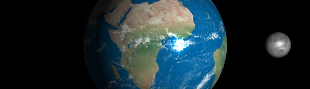
Now that we’ve seen how we can use textures, materials and lighting to render the objects in our scene, let’s examine an example that renders the moon rotating around the earth. The objects are realistically lit by a point-light that represents the sun.
In the rest of this article, I will assume you have already read the previous article titled [Introduction to OpenGL and GLSL]. If not, take a moment to read through that article before you continue with this one.
Shaders
Before we start with creating an application to interact with the shaders, let’s first define a vertex shader and a fragment shader that we can use in our application.
Vertex Shader
First we’ll define the vertex shader that will be used to transform the vertices of our geometry into clip-space so that they can be consumed by the rasterizer.
The lighting functions will be defined in the fragment shader later. One important thing to remember is that in order to perform proper lighting, all vectors and positions must be in the same “space”. Which space you want to perform lighting in is your choice but it should be consistent. For this demo, I choose to compute the lighting in world-space but it is also possible to performing the lighting in object-space, light-space, or view-space.
In order to perform the lighting in world-space, you must transform the vertex position and vertex normal into world-space in the vertex shader and pass the world-space attributes to the fragment shader. In addition to this, you must make sure that you provide the eye position (camera’s position) and the light’s position in world-space in the fragment shader.
First, let’s take a look at the vertex shader:
12345678910111213141516171819202122#version 330 corelayout(location=0) in vec3 in_position;layout(location=2) in vec3 in_normal;layout(location=8) in vec2 in_texcoord;out vec4 v2f_positionW; // Position in world space.out vec4 v2f_normalW; // Surface normal in world space.out vec2 v2f_texcoord;// Model, View, Projection matrix.uniform mat4 ModelViewProjectionMatrix;uniform mat4 ModelMatrix;void main(){gl_Position = ModelViewProjectionMatrix * vec4(in_position, 1);v2f_positionW = ModelMatrix * vec4(in_position, 1);v2f_normalW = ModelMatrix * vec4(in_normal, 0);v2f_texcoord = in_texcoord;}I won’t describe every line here as this was already described in the previous article titled [Introduction to OpenGL and GLSL]. What may be unfamiliar is the code on line 19 and 20. Since we will be performing the lighting calculations in the fragment shader in world-space, you must transform the vertex’s object-space position and surface normal into world-space by multiplying these attributes by the object’s model (or world) matrix.
The texture coordinate is not used for lighting calculations so it is simply passed-through as-is to the fragment shader.
Fragment Shader
The fragment shader is slightly more complicated. It accepts the vertex attributes from the vertex shader in addition to uniform variables that are used to define the light and material properties that will be used to correctly light our object.
First let’s take a look at the input variables.
1234567891011121314151617181920#version 330 corein vec4 v2f_positionW; // Position in world space.in vec4 v2f_normalW; // Surface normal in world space.in vec2 v2f_texcoord;uniform vec4 EyePosW; // Eye position in world space.uniform vec4 LightPosW; // Light's position in world space.uniform vec4 LightColor; // Light's diffuse and specular contribution.uniform vec4 MaterialEmissive;uniform vec4 MaterialDiffuse;uniform vec4 MaterialSpecular;uniform float MaterialShininess;uniform vec4 Ambient; // Global ambient contribution.uniform sampler2D diffuseSampler;layout (location=0) out vec4 out_color;The first few input variables on lines 3-5 are passed from the vertex shader to the fragment shader.
On line 7, the world-space eye position is assigned to the EyePosW uniform variable by the application. This is simply the position of the camera in world-space.
For point-lights, we need to know the world-space position of the light source. This value is stored in the LightPosW uniform variable.
For simplicity, we will assume that the diffuse contribution and the specular contribution of the light source are the same and we will store these values in a single uniform variable called LightColor.
On lines 11-14, the material properties are defined. For this shader, we’ll define the emissive, diffuse, specular, and shininess material properties.
For simplicity, I only define a single global ambient term. For you own lighting shaders, you may choose to separate the global, per-light, and material ambient values.
On line 18, a single uniform sampler is used to fetch a texel from the primary texture that is associated with the object being rendered.
On line 20, we define the only output parameter from our shader. The final fragment color which is mapped to the first color buffer in the active framebuffer (there is only one color buffer in the default framebuffer so we could omit the layout specification in this case).
Now let’s see how we implement the lighting equation for each fragment.
123456789101112131415161718192021void main(){// Compute the emissive term.vec4 Emissive = MaterialEmissive;// Compute the diffuse term.vec4 N = normalize( v2f_normalW );vec4 L = normalize( LightPosW - v2f_positionW );float NdotL = max( dot( N, L ), 0 );vec4 Diffuse = NdotL * LightColor * MaterialDiffuse;// Compute the specular term.vec4 V = normalize( EyePosW - v2f_positionW );vec4 H = normalize( L + V );vec4 R = reflect( -L, N );float RdotV = max( dot( R, V ), 0 );float NdotH = max( dot( N, H ), 0 );vec4 Specular = pow( RdotV, MaterialShininess ) * LightColor * MaterialSpecular;out_color = ( Emissive + Ambient + Diffuse + Specular ) * texture( diffuseSampler, v2f_texcoord );}On line 25, the materials emissive contribution is simply assigned to the Emissive local variable. Since the emissive term simply adds lighting when otherwise no lighting is present, the emissive term is not affected by the position of the light or the position of the viewer.
Next, the diffuse contribution is computed. The diffuse contribution is brightest when the surface normal \(\mathbf{N}\) and the light vector \(\mathbf{L}\) are pointing in the same direction (parallel) and it steadily falls-off as the angle between these two vectors increases. This is determined by the cosine angle (NdotL) between these two vectors. If the angle between them is 0, the cosine angle is 1 (brightest). As the angle between them increases, the cosine angle decreases until the two vectors are orthogonal in which case the cosine angle between them becomes 0 and no lighting contribution should occur. If \(\mathbf{N}\) and \(\mathbf{L}\) are pointing in opposite directions, then the cosine angle becomes negative but since we don’t want to have negative colors, we simply clamp the cosine angle to 0 using the max function.
In the next section, the specular term is computed. In this fragment program, I am computing the specular contribution using the Phong lighting model using \(\mathbf{R}\cdot\mathbf{V}\) and the Blinn-Phong model using \(\mathbf{N}\cdot\mathbf{H}\). To see the difference between these two lighting models, replace the RdotV on line 39 with NdotH.
On line 41, the final fragment color is computed by summing the lighting contributions and modulating it by the texture color of the object. The texture color is fetched from the texture using the special texture function. The first parameter to this function is the sampler that is associated with the texture unit that the object’s texture is bound to. The second parameter is the texture coordinates that are passed directly from the vertex shader.
This shader only computes the lighting contribution of a single light source. If you want to define more lights, you can simply create a for-loop around the diffuse and specular lighting calculations and change the LightPosW and the LightColor uniform variables to be arrays. The final Diffuse and Specular values will be the sum of all Diffuse and Specular contributions for all lights in the scene.
Next, we’ll see how we can create an application that can render a scene using these shaders.
Initialize GLUT and GLEW
Similar to the previous article titled [Introduction to OpenGL and GLSL], I will be using FreeGLUT and GLEW to initialize the OpenGL context and extensions. Please refer to that article for full details about these functions.
Loading Textures
We’ll use the SOIL library to load the textures used by this demo. We’ll also specify a few texture properties after the texture has been loaded.
If you are using Visual Studio 2012 and a forward-compatible context, make sure you use my version of SOIL and not the one from the SOIL website.
1234567891011GLuint LoadTexture( const std::string& file ){GLuint textureID = SOIL_load_OGL_texture( file.c_str(), SOIL_LOAD_AUTO, SOIL_CREATE_NEW_ID, SOIL_FLAG_MIPMAPS );glTexParameteri( GL_TEXTURE_2D, GL_TEXTURE_MIN_FILTER, GL_LINEAR_MIPMAP_LINEAR );glTexParameteri( GL_TEXTURE_2D, GL_TEXTURE_MAG_FILTER, GL_LINEAR );glTexParameteri( GL_TEXTURE_2D, GL_TEXTURE_WRAP_S, GL_REPEAT );glTexParameteri( GL_TEXTURE_2D, GL_TEXTURE_WRAP_T, GL_REPEAT );glBindTexture( GL_TEXTURE_2D, 0 );return textureID;}The SOIL_load_OGL_texture method can be used to load a texture and generate an OpenGL texture object that can then be used to texture the objects in our scene.
We also want to specify the texture filtering mode to GL_LINEAR_MIPMAP_LINEAR for the GL_TEXTURE_MIN_FILTER GL_LINEAR for the GL_TEXTURE_MAG_FILTER. We set the GL_TEXTURE_WRAP_* to GL_REPEAT to avoid seams appearing in our object.
On line 240, the default texture object ID of 0 is bound to the GL_TEXTURE_2D texture target and thus un-binding any previously bound texture object.
Creating a Sphere
Since all of the objects in our scene (the earth, the moon, and the sun) can all be represented by a sphere, we will generate a single sphere using a Vertex Array Object and use it to render each object in the scene.
I will create a procedural sphere that contains the texture coordinates and the vertex normals that are necessary to render the objects with lighting and texture.
I will describe this function in three parts:
- Setting up the vertex attributes
- Setting up the index buffer
- Setting up the Vertex Array Object
Vertex Attributes
First we’ll setup the vertex attributes for the sphere. Each vertex of the sphere will have three attributes: position, normal, and texture coordinate. The sphere will be centered at the origin (0, 0, 0) and have a specific radius. The number of segments along the principal axis of the sphere is determined by the stacks parameter and the number of segments around the circumference of each stack is determined by the slices parameter.
A wireframe view of our sphere may look something like the image shown below.

Wireframe sphere
The sphere’s principal axis goes from one pole to the other. The stacks traverse the principal axis and the slices go around the stacks.
123456789101112131415161718192021222324252627282930313233GLuint SolidSphere( float radius, int slices, int stacks ){using namespace glm;using namespace std;const float pi = 3.1415926535897932384626433832795f;const float _2pi = 2.0f * pi;vector<vec3> positions;vector<vec3> normals;vector<vec2> textureCoords;for( int i = 0; i <= stacks; ++i ){// V texture coordinate.float V = i / (float)stacks;float phi = V * pi;for ( int j = 0; j <= slices; ++j ){// U texture coordinate.float U = j / (float)slices;float theta = U * _2pi;float X = cos(theta) * sin(phi);float Y = cos(phi);float Z = sin(theta) * sin(phi);positions.push_back( vec3( X, Y, Z) * radius );normals.push_back( vec3(X, Y, Z) );textureCoords.push_back( vec2(U, V) );}}In this function, the sphere’s local Y-axis is the principal axis. If you want to use a different axis as the principal axis, simply swap the Y component with the component of the principal axis (for example the Z component).
Index Buffer
Now we have the vertex attributes for our sphere but we cannot simply render the vertices in this order (unless we only want to render points) because we must pass the sphere geometry to the GPU using triangles, we need to build an index buffer that defines the order in which to send the vertices to the GPU. We must also make sure that the ordering of the vertices in each triangle are correctly wound using a counter-clockwise winding order so that the outside of the sphere is not culled when using back-face culling.
12345678910111213// Now generate the index buffervector<GLuint> indicies;for( int i = 0; i < slices * stacks + slices; ++i ){indicies.push_back( i );indicies.push_back( i + slices + 1 );indicies.push_back( i + slices );indicies.push_back( i + slices + 1 );indicies.push_back( i );indicies.push_back( i + 1 );}Each face of the sphere consists of 2 triangles. An upper triangle and a lower triangle. Each iteration through this loop will create 2 triangles for each face of our sphere. If you change the principal axis as suggested in the previous step, make sure you change the order that the vertices are pushed in the index buffer to match. For example, if you make the Z axis the principal axis, swap the 2nd and 3rd indices for each triangle in this method.
The final step is to create the Vertex Array Object that encapsulates the sphere’s vertex attributes and index buffer.
Vertex Array Object
In this phase, we’ll create a Vertex Array Object (VAO) and bind the three vertex attributes and the index buffer to the VAO for easy rendering of our sphere.
12345678910111213141516171819202122232425262728293031GLuint vao;glGenVertexArrays( 1, &vao );glBindVertexArray( vao );GLuint vbos[4];glGenBuffers( 4, vbos );glBindBuffer( GL_ARRAY_BUFFER, vbos[0] );glBufferData( GL_ARRAY_BUFFER, positions.size() * sizeof(vec3), positions.data(), GL_STATIC_DRAW );glVertexAttribPointer( POSITION_ATTRIBUTE, 3, GL_FLOAT, GL_FALSE, 0, BUFFER_OFFSET(0) );glEnableVertexAttribArray( POSITION_ATTRIBUTE );glBindBuffer( GL_ARRAY_BUFFER, vbos[1] );glBufferData( GL_ARRAY_BUFFER, normals.size() * sizeof(vec3), normals.data(), GL_STATIC_DRAW );glVertexAttribPointer( NORMAL_ATTRIBUTE, 3, GL_FLOAT, GL_TRUE, 0, BUFFER_OFFSET(0) );glEnableVertexAttribArray( NORMAL_ATTRIBUTE );glBindBuffer( GL_ARRAY_BUFFER, vbos[2] );glBufferData( GL_ARRAY_BUFFER, textureCoords.size() * sizeof(vec2), textureCoords.data(), GL_STATIC_DRAW );glVertexAttribPointer( TEXCOORD0_ATTRIBUTE, 2, GL_FLOAT, GL_FALSE, 0, BUFFER_OFFSET(0) );glEnableVertexAttribArray( TEXCOORD0_ATTRIBUTE );glBindBuffer( GL_ELEMENT_ARRAY_BUFFER, vbos[3] );glBufferData( GL_ELEMENT_ARRAY_BUFFER, indicies.size() * sizeof(GLuint), indicies.data(), GL_STATIC_DRAW );glBindVertexArray( 0 );glBindBuffer( GL_ARRAY_BUFFER, 0 );glBindBuffer( GL_ELEMENT_ARRAY_BUFFER, 0 );return vao;}In this case, we are using packed arrays for our data. Each vertex attribute has it’s own Vertex Buffer Object (VBO). In order to define our VAO, we need four VBO’s. Three for the vertex attributes and one for the index buffer.
To copy the attributes to the VBO’s we first bind a VBO to the GL_ARRAY_BUFFER target and copy the data to the VBO using the glBufferData method.
We must also bind the generic vertex attributes to the correct buffer using the glVertexAttribPointer method and enable the generic vertex attribute using the glEnableVertexAttribArray method.
The constants POSITION_ATTRIBUTE, NORMAL_ATTRIBUTE, and TEXCOORD0_ATTRIBUTE are defined in the application to match the layout locations defined in the vertex shader (POSITION_ATTRIBUTE -> 0, NORMAL_ATTRIBUTE -> 2, TEXCOORD0_ATTRIBUTE -> 8). If you are wondering how I came up with these numbers, see http://http.developer.nvidia.com/Cg/glslv.html
Main
The main entry point for our application will initialize OpenGL, load the resources we need and query for the uniform locations in the shader program.
In the first part of the main function, we will initialize some variables and initialize OpenGL. Since this part of the function is identical to that of the previous article titled [Introduction to OpenGL and GLSL] I will not go into details about these functions here. For completeness, I will simply show the code.
1234567891011int main( int argc, char* argv[] ){g_PreviousTicks = std::clock();g_A = g_W = g_S = g_D = g_Q = g_E = 0;g_InitialCameraPosition = glm::vec3( 0, 0, 100 );g_Camera.SetPosition( g_InitialCameraPosition );g_Camera.SetRotation( g_InitialCameraRotation );InitGL(argc, argv);InitGLEW();In this case, we initialize the camera to be 100 units in the Z axis. Otherwise the rest of this code is identical to the code in the [Introduction to OpenGL and GLSL] article.
In the next section of the main function, we will load the textures that will be used and load the simpleShader shader program that was shown in the [Introduction to OpenGL and GLSL] article.
123456789101112131415g_EarthTexture = LoadTexture( "../data/Textures/earth.dds" );g_MoonTexture = LoadTexture( "../data/Textures/moon.dds" );GLuint vertexShader = LoadShader( GL_VERTEX_SHADER, "../data/shaders/simpleShader.vert" );GLuint fragmentShader = LoadShader( GL_FRAGMENT_SHADER, "../data/shaders/simpleShader.frag" );std::vector<GLuint> shaders;shaders.push_back(vertexShader);shaders.push_back(fragmentShader);g_SimpleShaderProgram = CreateShaderProgram( shaders );assert( g_SimpleShaderProgram );// Retrieve the location of the color uniform variable in the simple shader program.g_uniformColor = glGetUniformLocation( g_SimpleShaderProgram, "color" );On lines 337 and 338, the two textures which will be used to render the earth and the moon in our scene are loaded. The texture I use for this demo were downloaded from Tom Patterson, www.shadedrelief.com. I resized the images and converted them to DDS for faster loading and rendering.
On lines 340 and 341, the vertex and fragment shaders are loaded and on line 347 the shader program is created from these shaders.
On line 351, the location of the color uniform variable defined in the simpleShader program is queried.
The simpleShader shader program was explained in full detail in the [Introduction to OpenGL and GLSL] article so I will not explain its functionality here again. As well as the LoadShader and CreateShaderProgram functions were also explained in that article so they will not be explained here again.
Next we’ll load the textureLit vertex and fragment shaders and query for the uniform locations in that shader program.
1234567891011121314151617181920212223242526272829vertexShader = LoadShader( GL_VERTEX_SHADER, "../data/shaders/texturedDiffuse.vert" );fragmentShader = LoadShader( GL_FRAGMENT_SHADER, "../data/shaders/texturedDiffuse.frag" );shaders.clear();shaders.push_back(vertexShader);shaders.push_back(fragmentShader);g_TexturedDiffuseShaderProgram = CreateShaderProgram( shaders );assert( g_TexturedDiffuseShaderProgram );g_uniformMVP = glGetUniformLocation( g_TexturedDiffuseShaderProgram, "ModelViewProjectionMatrix" );g_uniformModelMatrix = glGetUniformLocation( g_TexturedDiffuseShaderProgram, "ModelMatrix" );g_uniformEyePosW = glGetUniformLocation( g_TexturedDiffuseShaderProgram, "EyePosW" );// Light properties.g_uniformLightPosW = glGetUniformLocation( g_TexturedDiffuseShaderProgram, "LightPosW" );g_uniformLightColor = glGetUniformLocation( g_TexturedDiffuseShaderProgram, "LightColor" );// Global ambient.g_uniformAmbient = glGetUniformLocation( g_TexturedDiffuseShaderProgram, "Ambient" );// Material properties.g_uniformMaterialEmissive = glGetUniformLocation( g_TexturedDiffuseShaderProgram, "MaterialEmissive" );g_uniformMaterialDiffuse = glGetUniformLocation( g_TexturedDiffuseShaderProgram, "MaterialDiffuse" );g_uniformMaterialSpecular = glGetUniformLocation( g_TexturedDiffuseShaderProgram, "MaterialSpecular" );g_uniformMaterialShininess = glGetUniformLocation( g_TexturedDiffuseShaderProgram, "MaterialShininess" );glutMainLoop();}On lines 353 and 354 we load the vertex and fragment shaders that were shown earlier and on line 360 we create the shader program that links the vertex and fragment shaders.
On lines 363-378 the uniform variables defined in the shader program are queried.
And on line 380, the main loop is kicked-off.
Render the Scene
To render this scene, we’ll draw 3 spheres. The first sphere will represent the sun. This will be an unlit white sphere that will rotate about 90,000 Km around the center of the scene. The position of the only light in the scene will be the same as the object that represents the sun.
The Earth is placed at the center of the scene. The earth rotates around its poles, but its positions stays fixed at the center of the scene (the Earth will not be translated).
The final object will be the moon. The moon appears to rotate around the earth but at a distance of 60,000 Km away from the earth.
In this scene, we make the agreement that 1 unit is approximately 1,000 Km. Although the units used are completely arbitrary, it makes sense to choose the units that are used in reality without requiring infinite depth buffer range. For example a common unit of measurement is 1 unit is equivalent to 1 meter when creating a first-person shooter.
In the first part of the render function, we will create a sphere VAO that can be used to render the sun, earth, and moon.
123456789void DisplayGL(){int slices = 32;int stacks = 32;int numIndicies = ( slices * stacks + slices ) * 6;if ( g_vaoSphere == 0 ){g_vaoSphere = SolidSphere( 1, slices, stacks );}The sphere VAO is created from a sphere with 32 slices and 32 stacks. Of course you can create a more detailed sphere with more slices and stacks if you think this sphere does not have enough detail but for my purposes this seems to be enough. If I was ambitious, I would have the SolidSphere function return a sphere object that stores the index count, and the ID’s of the internal VBOs that are used to store the geometry for the sphere but that is not required for the minimal implementation here. I encourage you to create a sphere object on your own which encapsulates the sphere data.
The next part of the render function will setup the uniform properties in the shader and render the sun, earth, and moon. Let’s first draw the sun using the SimpleShader shader program (since the sun is not textured or lit, we do not need to use the TextureLit shader program for this).
1234567891011121314151617const glm::vec4 white(1);const glm::vec4 black(0);const glm::vec4 ambient( 0.1f, 0.1f, 0.1f, 1.0f );glClear(GL_COLOR_BUFFER_BIT|GL_DEPTH_BUFFER_BIT);// Draw the sunglBindVertexArray(g_vaoSphere);glUseProgram( g_SimpleShaderProgram );glm::mat4 modelMatrix = glm::rotate( glm::radians(g_fSunRotation), glm::vec3(0,-1,0) ) * glm::translate(glm::vec3(90,0,0));glm::mat4 mvp = g_Camera.GetProjectionMatrix() * g_Camera.GetViewMatrix() * modelMatrix;GLuint uniformMVP = glGetUniformLocation( g_SimpleShaderProgram, "MVP" );glUniformMatrix4fv( uniformMVP, 1, GL_FALSE, glm::value_ptr(mvp) );glUniform4fv(g_uniformColor, 1, glm::value_ptr(white) );glDrawElements( GL_TRIANGLES, numIndicies, GL_UNSIGNED_INT, BUFFER_OFFSET(0) );On lines 409-411 a few constant variables are defined. These values will be used to set the uniform variables in the shaders.
On line 413 the color buffer and the depth buffer of the currently bound framebuffer is cleared.
On line 416 the VAO for the sphere object is bound. This sphere object will be used to render the sun, earth and moon so we don’t need to unbind it again until the end of the render function.
The sun is going to be rendered using a simple color shader. No lighting or texturing will be applied to the sun. It is simply a white ball in space. To render the sun, we bind the simple shader program on line 418.
To render the sun, we need to set the MVP and the color uniform variables that are defined in the shader program. To set a matrix uniform, we use the glUniformMatrix4fv and to set a 4-component vector uniform variable we use the glUniform4fv.
On line 419, the world-matrix for the sun is computed separately because we will use the world position of the sun to set the position of the light source in the next steps.
On line 425 the sphere representing the sun is rendered using the glDrawElements method.
Next, we will draw the earth.
123456789101112131415161718192021222324// Draw the earth.glBindTexture( GL_TEXTURE_2D, g_EarthTexture );glUseProgram( g_TexturedDiffuseShaderProgram );// Set the light position to the position of the Sun.glUniform4fv( g_uniformLightPosW, 1, glm::value_ptr(modelMatrix[3]) );glUniform4fv( g_uniformLightColor, 1, glm::value_ptr(white) );glUniform4fv( g_uniformAmbient, 1, glm::value_ptr(ambient) );modelMatrix = glm::rotate( glm::radians(g_fEarthRotation), glm::vec3(0,1,0) ) * glm::scale(glm::vec3(12.756f) );glm::vec4 eyePosW = glm::vec4( g_Camera.GetPosition(), 1 );mvp = g_Camera.GetProjectionMatrix() * g_Camera.GetViewMatrix() * modelMatrix;glUniformMatrix4fv( g_uniformMVP, 1, GL_FALSE, glm::value_ptr(mvp) );glUniformMatrix4fv( g_uniformModelMatrix, 1, GL_FALSE, glm::value_ptr(modelMatrix) );glUniform4fv( g_uniformEyePosW, 1, glm::value_ptr( eyePosW ) );// Material properties.glUniform4fv( g_uniformMaterialEmissive, 1, glm::value_ptr(black) );glUniform4fv( g_uniformMaterialDiffuse, 1, glm::value_ptr(white) );glUniform4fv( g_uniformMaterialSpecular, 1, glm::value_ptr(white) );glUniform1f( g_uniformMaterialShininess, 50.0f );glDrawElements( GL_TRIANGLES, numIndicies, GL_UNSIGNED_INT, BUFFER_OFFSET(0) );To draw the earth, we need to bind the earth texture to the first active texture unit. By default, the active texture unit is texture unit 0 and the uniform texture sampler in the textured diffuse shader program has a default value of 0 so we don’t need to explicitly set the value of the uniform sampler in the shader program to 0. It is sufficient to simply bind the texture to the GL_TEXTURE_2D texture target.
On line 429, we set the active shader program to be that of the textured and lit shader program that we compiled in the main function.
On line 432-434 we set the uniform variables in the shader. The light position in world space is the position of the sun we just rendered which is simply the 3rd column of the model matrix that was set on line 419. The color of the light is set to white on line 433 and the global ambient contribution is set on line 434.
On lines 436 the earth’s model matrix is computed. The model matrix is required as a separate parameter to the shader program because we will use it to transform the model’s vertex position and vertex normal into world space.
On line 437 the eye position in world space computed from the camera’s world position. The GetPosition function of the camera class returns a 3-component vector but our shader expects a 4-component vector so we need to cast the camera’s position to a 4-component vector by appending a 1 to the w-component so that it acts like a point in 3D space and not a direction vector.
On line 438 the model-view-projection matrix is computed. This matrix is used to transform the vertex position directly into clip-space.
On lines 440-442 the correct uniform variables in the shader program are set.
On lines 445-448 the uniform variables for the material properties are set. You’ll notice that the material shininess is set to 50.0. This will produce a rather bright specular highlight on the surface of the earth.
On line 450, we render the earth using the glDrawElements as before.
Next we draw the moon which is pretty much identical to rendering the earth except with a different model matrix, texture, and some material properties.
123456789101112131415// Draw the moon.glBindTexture( GL_TEXTURE_2D, g_MoonTexture );modelMatrix = glm::rotate( glm::radians(g_fSunRotation), glm::vec3(0,1,0) ) * glm::translate(glm::vec3(60, 0, 0) ) * glm::scale(glm::vec3(3.476f));mvp = g_Camera.GetProjectionMatrix() * g_Camera.GetViewMatrix() * modelMatrix;glUniformMatrix4fv( g_uniformMVP, 1, GL_FALSE, glm::value_ptr(mvp) );glUniformMatrix4fv( g_uniformModelMatrix, 1, GL_FALSE, glm::value_ptr(modelMatrix) );glUniform4fv( g_uniformMaterialEmissive, 1, glm::value_ptr(black) );glUniform4fv( g_uniformMaterialDiffuse, 1, glm::value_ptr(white) );glUniform4fv( g_uniformMaterialSpecular, 1, glm::value_ptr(white) );glUniform1f( g_uniformMaterialShininess, 5.0f );glDrawElements( GL_TRIANGLES, numIndicies, GL_UNSIGNED_INT, BUFFER_OFFSET(0) );Besides a different texture, model matrix and duller specular highlight, this is the same as the earth rendering code. I’ll spare you the details.
At the end of the render function, we should not forget to unbind (deactivate) the resources used.
123456glBindVertexArray(0);glUseProgram(0);glBindTexture( GL_TEXTURE_2D, 0 );glutSwapBuffers();}The VAO, shader program, and texture should be unbound so that we leave the OpenGL state machine the way we found it.
On line 472, the front and back buffers are swapped so that we can see what we just rendered.
View the Demo
The demo below demonstrates the example shown in this article. The demo uses WebGL to render the scene. The WebGL demo will render in the latest FireFox browser as well as the latest Chrome browser. If you are using Internet Explorer however, then you are probably not going to see the beautiful demo but instead you will see the YouTube video.
Texture and Lighting Demo
Download the Demo
You can download the source code and project files for the demo shown in this article here:
 OpenGL_TexturingAndLighting.zip
Exercises
- Change the fragment shader so that the specular component is calculated using the half-angle vector instead of the reflected vector. What is the effect of this change and why?
- Download the Land/Water mask from http://www.shadedrelief.com/natural3/pages/extra.html and use the mask to determine the shininess of the surface of the earth. For water surfaces use a shininess value of 100 and for the land use a shininess value of 10.
- Download the Earth at Night texture from http://www.shadedrelief.com/natural3/pages/textures.html and blend the daytime and nightime maps based on the diffuse contribution of the light.
- Download a cloud map from http://www.shadedrelief.com/natural3/pages/clouds.html and render a slightly larger sphere over the earth. Use transparent blending (using the cloud map to determine the alpha value) to blend the clouds over the earth rendering.
- Texture the sun with a sun texture map.
- Download the Starfield backdrop from http://www.shadedrelief.com/natural3/pages/extra.html and render it onto a unit sphere that is placed at the position of the camera. If you use the same sphere as is used to render the sun, earth, and moon, make sure your reverse the winding order using the glFrontFace method or use glCullFace to draw the inside of the sphere instead of the outside. Also don’t forget to disable depth writes when you render the sphere map so that the sun, earth, and moon are still drawn correctly.
- Texture the sun with a sun texture map.
References
Benstead, Luke with Astle, D. and Hawkins, K. (2009). Beginning OpenGL Game Programming. 2nd. ed. Boston, MA: Course Technology.")
Beginning OpenGL Game Programming - Second Edition (2009)
Mason Woo, Jackie Neider, Tom Davies, Dave Shreiner (1999). OpenGL Programming Guide. 3rd. ed. Massachusetts, USA: Addison Wesley.
OpenGL Programming Guide - 3rd Edition
OpenGL 2.1 Reference Pages [online]. (1991-2006) [Accessed 27 January 2012]. Available from: http://www.opengl.org/sdk/docs/man/. The Earth textures were retrieved from http://www.shadedrelief.com/natural3/pages/textures.html. Special thanks to Tom Patterson for providing these textures. The Moon textures were retrieved from http://www.buining.com/. Special thanks to Jan-Herman Buining for providing these textures.


")

Finally, a sphere tutorial that works.
Thank you very much!
Thanks a lot!! very complete
Thanks for posting a great tutorial! I implemented in OpenGL 2.1.
One question: It looks like I’m looking at the back of the texture. In other words, Florida is west of California. I have tried reversing the normals, the windings, and setting the v2f_texcoord to vec2(1.0, 1.0) – v2f_texcoord. The issue persists. I can’t wrap my head around this. Insight?
If your texture is flipped around on the horizontal axis (X-axis), then the texture would appear upside-down. In this case you would need to flip the V texture coordinate (in a UV texture coordinate system).
texCoord.v = 1 - texcord.v(Assuming normalized texture coordinates in the range 0 .. 1).
If the texture is flipped around the vertical axis (Y-axis), then the texture would appear “backwards” (as in your case). In this case you would need to flip the U texture coordinate.
texCoord.u = 1 - texCoord.uYou may want to try:
texCoord = vec2( 0, 1 ) - texCoordor
texCoord = vec2( 1, 0 ) - texCoorddepending on which axis appears flipped.
It is unlikely that you want to flip both coordinates (which is what happens in your case) since this will flip it in both axes.
I hope this helps!
Thanks for getting back to me. I was burning the midnight oil. My apologies.
What concerned me is I am using your texture image. It turns out I was I was using a left-hand projection.
Hello !
Thank you for your wonderful work ! I’m very new to programming, would you please give me some instructions on how to compile your program on a Mac OS, probably using Cmake ? I always encounter errors when compiling SOIL.
George,
I’m not that familiar with working on Mac OS but maybe if you can describe the errors you are encountering, it will be easier to help you fix them?